Preface
When reading federated learning papers, you often encounter a sentence: “Partition client data using a Dirichlet distribution and control the Non-IID degree with $\alpha$.” It looks like a ready-made experimental switch, but if you only remember that “the smaller $\alpha$ is, the more uneven the data is,” you easily miss critical details.
Is this probability vector assigning different labels to a client, or assigning different clients to a label? Is $\alpha$ the parameter for each coordinate, or the sum of parameters for all coordinates? Does the partitioning code inadvertently change the data volume per client? These questions all affect experimental results.
This article starts from the probability distribution itself and then provides a directly runnable data partitioning example. Here we discuss artificially constructed label heterogeneity, not a complete modeling of real-world federated data.
Why Simulate Non-IID?
Suppose the data of client $k$ comes from distribution $P_k(X,Y)$. When distributions differ across clients, their local optimization objectives may also differ:
Here, $\pi_k\ge0$, and $\sum_k\pi_k=1$; a common choice is weighting by the number of samples per client. Even if all clients start from the same model, after performing multiple steps of local training individually, the update directions may gradually diverge.
But Non-IID does not come in just one form:
| Difference | An Intuitive Example | Can Label-Only Partitioning Fully Simulate This? |
|---|---|---|
| Label Distribution Difference $P_k(Y)$ | Different ratios of cat vs. dog images on different devices | Yes, this dimension can be constructed |
| Conditional Feature Distribution Difference $P_k(X\mid Y)$ | For the same dog, different devices use different cameras to capture images | No, cannot fully simulate |
| Conditional Labeling Mechanism Difference $P_k(Y\mid X)$ | Different institutions adopt different labeling rules for similar samples | No, cannot fully simulate |
| Sample Size Difference $n_k$ | Active users vs. low-frequency users have different data volumes | May be simultaneously introduced by the partitioning process |
These descriptions are not entirely independent. For example, fixing the pools of samples for each category and changing label ratios can also alter the overall feature distribution of clients. In experiments, one should specify exactly what was constructed, rather than compressing all differences into a single “Non-IID” label.
Hsu et al. used the Dirichlet distribution to generate varying degrees of client label distributions to study the impact of such differences on FedAvg. It provides a useful experimental approach, but the meaning of its parameters must be read in conjunction with its specific construction. 1
What is the Dirichlet Distribution?
It Generates a Probability Vector
A $d$-dimensional Dirichlet random vector satisfies
where each $\alpha_i>0$. Its output is not a class label nor an integer sample count, but the proportion of each class or each client.
Let $\alpha_0=\sum_i\alpha_i$. Inside the simplex, its density is
Here, the density is defined relative to the $d-1$-dimensional coordinates, because the last component is determined by the preceding ones. In two dimensions, it degenerates to the Beta distribution; in three dimensions, each sample can be plotted as a point inside a triangle.
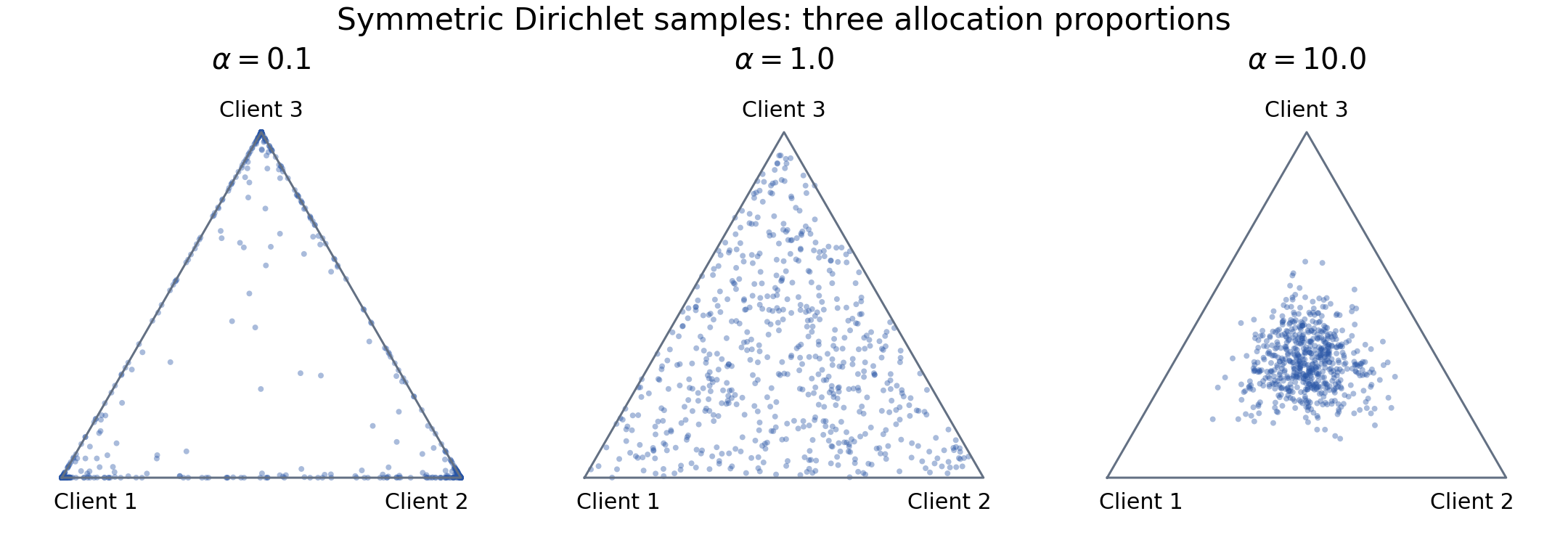
Each point represents a set of proportions summing to 1. Points near a vertex indicate one component dominates, while points near the center indicate the three components are roughly equal.
Definitions and sampling methods can be found in Stanford Course Notes2 and NumPy Documentation3. In the figure, $\alpha$ refers to the parameter for each coordinate.
Mean and Variance Are Two Different Things
The mean, variance, and covariance between different coordinates of the Dirichlet distribution are
Negative covariance is not surprising: since the sum of all proportions is fixed at 1, if one component grows larger, the others must yield space.
If symmetric parameters $\alpha_1=\cdots=\alpha_d=\alpha$ are used, then
Therefore, reducing $\alpha$ does not change the average proportion of each coordinate, but rather increases the fluctuation between a single sample and the average proportion. One sample might assign almost everything to the first component, while the next might assign almost everything to the third component.
- When $\alpha<1$, the distribution is more biased toward the boundaries of the simplex, making it likely that some components are very small while others dominate.
- When $\alpha=1$, the distribution is uniform over the simplex, but it does not output uniform proportions every time.
- When $\alpha>1$, the distribution is more concentrated toward the center; when $\alpha$ is very large, the proportions become closer to $1/d$.
This is a trend at the distribution level and does not guarantee that every small $\alpha$ sample is more skewed than every large $\alpha$ sample. Even when the probability vector is very close to uniform, allocating a finite number of samples still introduces fluctuations; a large $\alpha$ does not make every client’s empirical distribution exactly identical.
Single Coordinate Parameter vs. Total Concentration
The parameters can also be written as $\alpha_i=s m_i$, where $m_i>0$ and $\sum_i m_i=1$, so
$\mathbf m$ controls the center position, while $s$ controls the fluctuations around this center. A uniform center corresponds to $m_i=1/d$, in which case the parameter for each coordinate is $s/d$.
Therefore, the parameters $\operatorname{Dir}(\alpha,\ldots,\alpha)$ and $\operatorname{Dir}(\alpha\mathbf m)$ cannot be directly compared. The former has a total concentration of $d\alpha$, while the latter has a total concentration of $\alpha$. The paper by Hsu et al. uses the latter notation; when reproducing experiments, this distinction must be made explicit.
In Federated Learning, There Are Two Partitioning Directions
Assume there are $K$ clients and $C$ classes, with the sample count for class $c$ being $N_c$.
Direction 1: Generate Class Proportions for Each Client
For each client $k$, sample a $C$-dimensional vector:
This describes the class proportions the client is expected to hold. If the client requires a fixed number of $n_k$ samples, the integer counts for each class can then be determined.
The difficulty lies in the fact that the sum of demands across all clients may exceed the actual inventory of samples for a given class. If sampling independently from the class pool, one must clarify whether replacement is allowed; if not, supply-demand mismatches must be handled. Implementing balanced client sample sizes may also introduce additional constraints.
Direction 2: Generate Client Proportions for Each Class
For each class $c$, sample a $K$-dimensional vector:
In this way, all existing samples of each class can be distributed, and $\sum_kN_{kc}=N_c$. The final data volume for each client is $n_k=\sum_cN_{kc}$; for non-empty clients, their empirical label proportions are
Note that $r_{c,k}$ describes “the proportion of samples from class $c$ assigned to client $k$,” not “the proportion of class $c$ within client $k$.” Their normalization directions differ.
We adopt the second construction below. It preserves the total number of classes in the entire dataset but does not guarantee equal sample sizes per client, nor does it guarantee that every client has samples. When $\alpha$ is small, a client might receive samples from multiple classes or none at all; one cannot simply copy the “one client, one class” intuition from the first construction.
A Reproducible NumPy Implementation
The function below accepts 1D integer labels and returns the original sample indices held by each client. It first shuffles the indices for each class, uses Dirichlet to generate proportions, and then determines integer sample counts via the multinomial distribution.
| |
Here, we do not simply multiply the floating-point proportions by $N_c$ and floor the result, so there is no risk of “missing a few samples per class”; the sum of counts from the multinomial distribution exactly equals $N_c$. 4
An empty array is a valid partitioning result but cannot be directly fed into training pipelines that require non-empty datasets. If experiments disallow empty clients, one must redesign the allocation constraints or use resampling with a maximum count limit; these additional rules should be explicitly reported rather than silently discarding clients.
The label heatmap in the figure was generated using the same function: 20 clients, 10 classes, 500 samples per class, with a random seed of 42. Colors represent the class proportions within a non-empty client, and all panels use the same color scale.
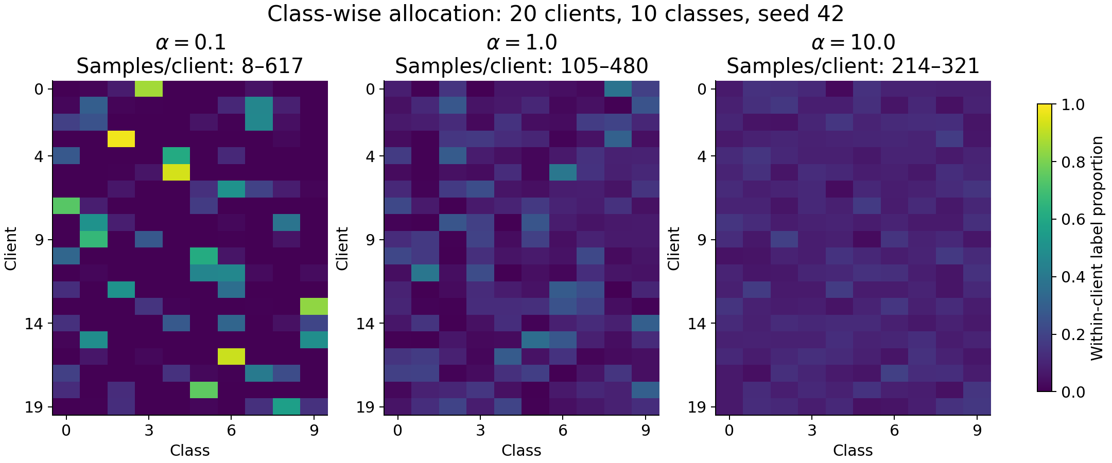
After assigning categories to clients, smaller alphas typically induce stronger label skew and may also alter the sample size per client. Empty clients, if any, are shown in gray.
What Else to Check When Running Experiments?
Do Not Just Save the Random Seed
Recording the random seed is useful, but one should also save the final list of client indices, the dataset version, the sample order, and the NumPy version. Changing the data loading order or the sequence of random number calls can cause the same seed to produce completely different partitions.
When comparing multiple algorithms under the same setting, try to reuse the same partition and report the mean and variance using multiple partition seeds. Do not mistake an accidentally easy partition for an algorithmic advantage.
Observe Label Skew and Sample Size Skew Separately
In addition to heatmaps, one should also statistics on the sample size, the number of non-empty classes, and label entropy for each client. For non-empty clients, label entropy can be written as
Here we use the natural logarithm; for a uniform coverage of $C$ classes, it equals $\log C$. Low entropy indicates more concentrated labels, but it does not fully describe differences between two clients: two clients may both have an entropy of 0 (each having only one class) while the classes themselves are completely different.
Accuracy weighted by sample size and accuracy averaged across clients answer different questions. The former favors overall sample performance, while the latter focuses on the experience of an average client; when $n_k$ differences are large, the two metrics can diverge significantly.
Be Careful About the Relationship Between Training, Validation, and Testing
You can manually split only the training set and retain an independent, fixed global test set; if you need to evaluate per-client local performance, you must explicitly define how local test data is generated. Real-world multi-user data should also be split by user or entity to avoid highly correlated samples from the same individual crossing between training and test sets.
Splitting training and validation data within pre-fixed client assignments, versus randomly splitting all samples first and then generating clients, may yield different evaluation targets. Both approaches must be clearly explained.
Comparative Experiments Must Report Full Configuration
At minimum, record the split direction, definition of the parameter vector, $K$, $C$, sample sizes for each class, random seed, integer allocation method, handling of empty clients, minimum sample size constraints, as well as client sampling and aggregation weights. Reporting only “$\alpha=0.5$” is insufficient for others to reproduce your experiment.
Conclusion
The role of the Dirichlet distribution is to provide a probability vector whose fluctuation level can be tuned. It allows us to construct label heterogeneity more conveniently, but $\alpha$ is not a universal difficulty scale that remains valid after removing dimensionality, allocation direction, and additional constraints.
What truly deserves scrutiny is the final client data: which classes went where, how many samples each client holds, and whose performance the evaluation metrics are actually measuring. Clearly documenting these details is more important than simply placing a single Non-IID parameter in an experimental table.
References and Further Reading
Sources: 5.
Hsu, Qi, and Brown: Measuring the Effects of Non-Identical Data Distribution for Federated Visual Classification. ↩︎
Stanford:Modelling Mixtures — the Dirichlet distribution。 ↩︎
NumPy: Generator.dirichlet and Generator.multinomial. ↩︎
NumPy: Generator.dirichlet and Generator.multinomial. ↩︎
Privacy Leakage in Deep Learning: Data remaining on clients does not imply that the transmitted updates lack sensitive information. ↩︎