hCaptcha Left-Flying Airplane Recognition: Image Processing Approach

My machine is a living life. I’ll prove it.

Introduction

hCaptcha has just received another update today, introducing a new tag that requires selecting in the sky left-flying airplanes.

Fortunately, however, every sample image contains an airplane, so this tag effectively removes one constraint, leaving only the two constraints of in the sky and flying left.

Main Method

First, let’s observe the images, still referring to the collected dataset¹. Besides the fact mentioned earlier that each sample image contains an airplane, if the airplane is in the sky, its background must be very “clean”. If it is not in the sky, it can basically be judged as being on the ground. Images on the ground also consist of multiple regions, such as lawns, airport runways, background forests, background skies, etc.

So, the key to distinguishing the first problem is the complexity of the background. How to do it?

My initial idea was to inherit the previous approach of color block filtering, but after dividing the color blocks, it was difficult to distinguish whether a block was an airplane or a background block, so it was discarded.

Then, I looked at most methods for removing sky backgrounds, which are basically based on threshold filtering in the HSV color space, followed by morphological operations like erosion and dilation for noise reduction. I tested it a few times myself, but the color range of the sky is slightly too large, containing blue, white, and yellow. More critically, it is very similar to the color of airplanes, as airplanes are mostly light colors like pale blue or white. This was also discarded.

I then thought that the shadow under the airplane would be black, so creating a superpixel smart selection based on black could work, but I don’t know how to implement it (x, so it was discarded.

Finally, the adopted solution was to use the contour line method Canny to find all contour lines, then set a threshold to determine if the airplane is in the sky based on the number of contour lines. If it is in the sky, the contour lines will be very simple, whereas if it is not in the sky, a large amount of chaotic lines will be added. Of course, this threshold was derived by randomly testing a few images, given the huge difference between the two cases. After such processing, the judgment accuracy approaches 100%.

Okay, one problem solved. Now, the remaining problem is: how to determine if the airplane is facing left?

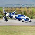
This really stumped me. Without using Deep Learning, it is indeed difficult, but there are some clever tricks. First, most airplanes are transport planes, fighters, or passenger jets; there are rarely propeller planes in the front, and I haven’t seen helicopters either. There are even WTF Airplanes like the one below (what the heck is this?)

Since that’s the case, these types of airplanes have a characteristic: “light head, heavy tail”. Besides the tail fin being heavier and the nose being pointed and lighter, the wings also point backward, so the “center of gravity” of the entire image should be biased towards the tail. I could determine the airplane’s direction based on 4 points: extreme left, extreme right, midpoint, and center of gravity.

Sounds scientific, right? However, the actual effect was not very good. The most critical issue is that airplanes have perspective relationships, so from the front view, the center of gravity might appear to be at the front. For example, if the nose is facing you, a large number of lines are drawn above the nose, while there are very few lines at the tail, making the center of gravity of the entire image appear at the front. Later, I wondered if I could fill the image, but the resulting contour lines were mostly not closed, making it difficult to fill the entire airplane (if that were possible, image segmentation would be simple).

Later, I had a sudden inspiration and took a different path. Still observing the contour lines drawn above, the nose, lacking complex elements, produces relatively “simple” contour lines, while the tail, due to components like “tail fins”, produces relatively “complex” ones. So how to measure this “simplicity” and “complexity”? Just sum them up… That’s right, in the end, I counted the non-zero pixels from x_min to x_min + left_threshold on the left (which are the contour line pixels) and compared them with the pixel count from x_max - left_threshold to x_max. Whichever is larger is the tail; if the right side is larger, then the nose is on the left. Unexpectedly, the final result was quite good, basically passing verification within 1-2 rounds.

Attached is the complete code for the test version

  1
  2
  3
  4
  5
  6
  7
  8
  9
 10
 11
 12
 13
 14
 15
 16
 17
 18
 19
 20
 21
 22
 23
 24
 25
 26
 27
 28
 29
 30
 31
 32
 33
 34
 35
 36
 37
 38
 39
 40
 41
 42
 43
 44
 45
 46
 47
 48
 49
 50
 51
 52
 53
 54
 55
 56
 57
 58
 59
 60
 61
 62
 63
 64
 65
 66
 67
 68
 69
 70
 71
 72
 73
 74
 75
 76
 77
 78
 79
 80
 81
 82
 83
 84
 85
 86
 87
 88
 89
 90
 91
 92
 93
 94
 95
 96
 97
 98
 99
100
101
102
103
104
105
106
107
108
109
110
111
112
113
114
115
116
117
118
119
120
121
122
123
124

from itertools import count
import cv2
import numpy as np
import matplotlib.pyplot as plt
from scipy import ndimage as ndi
from skimage.util import random_noise
from skimage import feature


class SkyLeftAirplaneChallenger:
    """A fast solution for identifying vertical rivers"""
    def __init__(self):
        self.flag = "skyleftairplane_model"
        self.sky_threshold = 1800
        self.left_threshold = 30
        self.debug = True

    @staticmethod
    def _remove_border(img):
        img[:, 1] = 0
        img[:, -2] = 0
        img[1, :] = 0
        img[-2, :] = 0
        return img

    def solution(self, img_stream, **kwargs) -> bool:  # noqa
        """Implementation process of solution"""
        img_arr = np.frombuffer(img_stream, np.uint8)
        img = cv2.imdecode(img_arr, flags=1)
        img = cv2.cvtColor(img, cv2.COLOR_BGR2GRAY)

        # cv2.imshow("img", img)
        # cv2.waitKey(0)

        edges1 = feature.canny(img)
        edges1 = self._remove_border(edges1)
        edges2 = feature.canny(img, sigma=3)
        edges2 = self._remove_border(edges2)

        # display results
        # fig, ax = plt.subplots(nrows=1, ncols=3, figsize=(8, 3))

        # ax[0].imshow(img, cmap='gray')
        # ax[0].set_title('noisy image', fontsize=20)

        # ax[1].imshow(edges1, cmap='gray')
        # ax[1].set_title(r'Canny filter, $\sigma=1$', fontsize=20)

        # ax[2].imshow(edges2, cmap='gray')
        # ax[2].set_title(r'Canny filter, $\sigma=3$', fontsize=20)

        # for a in ax:
        #     a.axis('off')

        # fig.tight_layout()
        # plt.show()

        # fill_plane = ndi.binary_fill_holes(edges1)

        # fig, ax = plt.subplots(figsize=(4, 3))
        # ax.imshow(fill_plane, cmap=plt.cm.gray)
        # ax.set_title('filling the holes')
        # ax.axis('off')
        # plt.show()
        # print(np.count_nonzero(edges1))
        # print(np.count_nonzero(edges2))

        if np.count_nonzero(edges1) > self.sky_threshold:
            if self.debug:
                print('[not in sky] ', end='')
            return False

        # get avg coordinate of edges where edges are not zero
        # avg_point = np.average(np.nonzero(edges1), axis=1)
        # print(avg_point)

        min_x = np.min(np.nonzero(edges1), axis=1)[1]
        max_x = np.max(np.nonzero(edges1), axis=1)[1]

        left_nonzero = np.count_nonzero(edges1[:, min_x:min(max_x, min_x + self.left_threshold)])
        right_nonzero = np.count_nonzero(edges1[:, max(min_x, max_x - self.left_threshold):max_x])

        # print(left_nonzero, right_nonzero)

        if left_nonzero > right_nonzero:
            if self.debug:
                print('[not turn left] ', end='')
            return False

        # mid_x = (min_x + max_x) / 2

        # print(min_x, max_x, mid_x, avg_point[0] < mid_x)

        # if avg_point[0] >= mid_x:
        #     return False

        # plt.show()
        return True


if __name__ == '__main__':
    import os
    import sys
    sys.path.append(os.path.dirname(os.path.dirname(os.path.abspath(__file__))))

    result_path = 'result.txt'
    if os.path.exists(result_path):
        os.remove(result_path)

    # result_file = open(result_path, 'w')
    result_file = sys.stdout

    base_path = os.path.join('..', 'database', 'airplane_in_the_sky_flying_left')
    image_list = os.listdir(base_path)
    # image_list.sort()
    for image_name in image_list:
        image_path = os.path.join(base_path, image_name)
        with open(image_path, "rb") as file:
            data = file.read()
        solution = SkyLeftAirplaneChallenger().solution(data)
        result_file.write(f'{image_name}: {solution}\n')
        result_file.flush()

    result_file.close()

Conclusion

To be honest, solving a high-quality image processing problem from hCaptcha every day still feels pretty cool hhhh.

However, through sharing by netizens, I have seen more problems solved using generative models. After all, they are paid to do this, and later some tasks can no longer be solved just by image processing, such as black-and-white striped cats that appeared in feedback for certain Tampermonkey plugins.

Just a clever workaround to meet each challenge.