The original article is in Chinese. The English version is automatically translated by AI.
Preface
In federated learning papers, the split often gets one sentence. Use Dirichlet sampling and vary $\alpha$ to control how non-IID the clients are. The easy part to remember is that smaller $\alpha$ gives more skew. When I try to reproduce the split, the missing details in that sentence are where I get stuck.
I start by asking what the proportions describe. Are they the classes within one client, or the clients that receive one class? Then I check whether $\alpha$ is the number on each coordinate or the sum across coordinates. And did the split change the number of samples per client too? All of that can affect the experiment.
So I want to go through the split from the beginning, then run an example and count what each client actually got. We’ll construct heterogeneity through the label proportions here. Real federated data can vary in the other ways below too.
Why Simulate Non-IID?
Think about one client first. Client $k$ gets its data from $P_k(X,Y)$. If another client’s data comes from a different distribution, it may be minimizing a different local objective.
Combine the clients’ objectives with weights satisfying $\pi_k\ge0$ and $\sum_k\pi_k=1$. A common choice is to weight by sample count. Everyone starts from the same model, but after a few steps on their own data, those updates can point in different directions.
When I hear non-IID, I like to line up a few small examples and see which difference we’re talking about.
| Difference | An Intuitive Example | Can Label-Only Partitioning Fully Simulate This? |
|---|---|---|
| Label Distribution Difference $P_k(Y)$ | Different ratios of cat vs. dog images on different devices | Yes, this dimension can be constructed |
| Conditional Feature Distribution Difference $P_k(X\mid Y)$ | For the same dog, different devices use different cameras to capture images | No, cannot fully simulate |
| Conditional Labeling Mechanism Difference $P_k(Y\mid X)$ | Different institutions adopt different labeling rules for similar samples | No, cannot fully simulate |
| Sample Size Difference $n_k$ | Active users vs. low-frequency users have different data volumes | May be simultaneously introduced by the partitioning process |
There’s a detail here that’s easy to miss. Keep the sample pool within each class fixed, then change the class proportions. A client’s overall feature distribution can change along with them. In an experiment I’d write down which part I actually changed.
Hsu and colleagues give an example to compare against. They vary client label distributions with Dirichlet sampling and look at what happens to FedAvg. When I get to the parameter they report, I go back to the split to see where it goes. 1
What is the Dirichlet Distribution?
It Generates a Probability Vector
Take one draw first. What we get is a $d$-dimensional vector whose entries add to one.
Each parameter satisfies $\alpha_i>0$. The draw tells us the shares to aim for. The class assignments and whole sample counts come when we use those shares in the split.
To work with the density, first add the parameters and call the total $\alpha_0=\sum_i\alpha_i$. Inside the simplex, the density is as follows.
If the density seems to be missing a dimension, remember that the last proportion is fixed by the earlier ones. That’s why it uses $d-1$ coordinates. With two entries this gives a beta distribution. With three, we can just plot each draw as a point in a triangle.
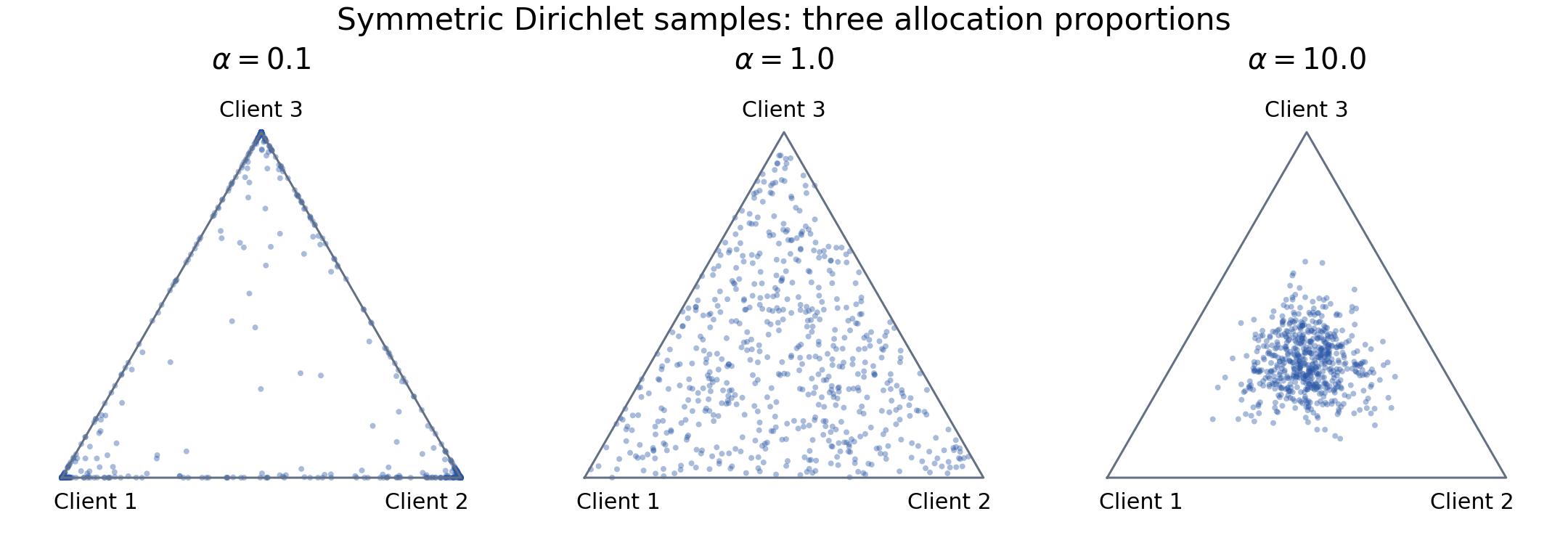
Each point represents a set of proportions summing to 1. Points near a vertex indicate one component dominates, while points near the center indicate the three components are roughly equal.
The $\alpha$ on the figure is the parameter on each coordinate. For the density or sampling details, see the Stanford notes2 and NumPy documentation3.
Mean and Variance Are Two Different Things
After looking at the plot, I want to know where the points are centered and how far they scatter. Start with the mean, variance, and covariance between coordinates.
I remember the negative sign in the covariance from the fixed total. If one share goes up, the others have to go down in total.
Now make the parameters simple and put the same number on every coordinate, $\alpha_1=\cdots=\alpha_d=\alpha$. The expressions are easier to read in that case.
So smaller $\alpha$ means individual draws can land farther from the mean. Imagine two draws in a row. The first could give nearly everything to the first entry, and the next could give it to the third. Under the distribution, the expectation is still the same for every entry.
- With $\alpha<1$, look at the three-coordinate plot above. Draws are more likely to crowd the triangle’s edges and corners, with some small shares and one that takes a lot.
- With $\alpha=1$, points are drawn uniformly from the simplex. That includes places near its boundary where the proportions can be quite different.
- With $\alpha>1$, the points cluster more toward the center. Increase $\alpha$ and each entry gets closer to $1/d$.
You see the trend best over many draws. A small $\alpha$ can still land near the middle, and a large $\alpha$ can land away from it. Then we have to assign whole samples. Even with a large $\alpha$, the empirical distributions on the clients can still fluctuate.
Single Coordinate Parameter vs. Total Concentration
If we want to choose the center first and then decide how much spread is around it, we can write the parameters as $\alpha_i=s m_i$, with $m_i>0$ and $\sum_i m_i=1$.
I read $\mathbf m$ as the center and $s$ as controlling the spread around it. For an equal-share center, take $m_i=1/d$, which gives $s/d$ on each coordinate.
This is why I look up the definition when two papers both report alpha. The parameters in $\operatorname{Dir}(\alpha,\ldots,\alpha)$ sum to $d\alpha$, while the total concentration in $\operatorname{Dir}(\alpha\mathbf m)$ is $\alpha$. Hsu and colleagues use the latter convention. I’d write down which one I used when reproducing the split.
In Federated Learning, There Are Two Partitioning Directions
Assume there are $K$ clients and $C$ classes, with the sample count for class $c$ being $N_c$.
Direction 1: Generate Class Proportions for Each Client
For the first approach, look from client $k$’s side. It draws a $C$-dimensional vector that says how much of each class it should get.
If that client needs exactly $n_k$ samples, use its proportions to decide how many to request from each class.
Add everyone’s requests at this point and a class can be oversubscribed. When drawing separately from each class pool, say whether the same sample can be picked again. If every sample is assigned only once, we have to handle that mismatch. If client sizes also need to match, add that constraint explicitly.
Direction 2: Generate Client Proportions for Each Class
Or reverse the order. Take the whole pool for class $c$ and ask where to send it. The draw now has $K$ entries, one for each client.
This way we can allocate the whole class pool, with $\sum_kN_{kc}=N_c$. Wait until all classes have been assigned to count each client’s total $n_k=\sum_cN_{kc}$. For a client with samples, we can then work out the share of each class it actually received.
I keep one sentence in mind for $r_{c,k}$. We’re holding the pool for class $c$ and asking what share goes to client $k$. To ask what share of client $k$ is class $c$, change the denominator to that client’s sample count.
I’ll use the second construction below and split one class at a time. The class totals add up, and we find out the client sizes at the end. At small $\alpha$, one client can get several classes while another ends up empty.
A Reproducible NumPy Implementation
Read the function in the same order. It takes a one-dimensional array of integer labels. For each class it shuffles the indices, draws Dirichlet shares, and uses a multinomial to turn those shares into whole sample counts. The result is a set of indices into the original data.
| |
Here’s where I check for missing samples. Multiply each share by $N_c$ and round it down and a few can be left over. With the multinomial counts, everything still adds up to $N_c$. 4
If one client comes back empty, pause before dropping it. It’s a possible outcome of the split. If training requires every client to have data, add an explicit allocation constraint or set a limit on redraws. Record whichever rule you used.
The figure shows one run of the same function. There are 20 clients and 10 classes, with 500 samples per class and seed 42. The colors show each class’s share within a nonempty client, with the same scale across panels.
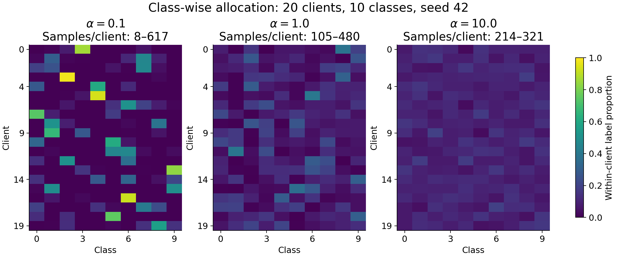
After assigning categories to clients, smaller alphas typically induce stronger label skew and may also alter the sample size per client. Empty clients, if any, are shown in gray.
What Else to Check When Running Experiments?
Do Not Just Save the Random Seed
To run on the same split next time, I’d save the indices the clients actually received. Record the seed too, along with the dataset and NumPy versions and the original sample order. A different load order or one extra random draw can produce another split from the same seed.
If I’m comparing algorithms I’d give them all the same partition first. Then repeat with several partition seeds and look at the mean and spread, so a single easy draw doesn’t get credited to the algorithm.
Observe Label Skew and Sample Size Skew Separately
After looking at the heatmap I usually count each client’s samples, its nonempty classes, and its label entropy. For a client with data, the entropy is given by the expression below.
This uses the natural logarithm and reaches $\log C$ for an even split over $C$ classes. Smaller values mean the labels are more concentrated. Picture one client getting only cats and another getting only dogs. Both entropies are zero, even though their labels are completely different.
When someone gives me an accuracy number I ask one more thing. Giving every sample equal weight and giving every client equal weight tell us different things. If $n_k$ varies a lot, check whether we’re describing performance over the samples or the experience of a typical client.
Be Careful About the Relationship Between Training, Validation, and Testing
We can hold an independent global test set fixed and split just the training data. To see how each client does locally, also explain how its test data was made. With real multi-user data, I’d split by user or subject so closely related examples from one person don’t land in both training and test.
Sometimes we assign clients first and split their data into training and validation. Sometimes we split the whole dataset before assigning clients. Changing that order can change what the evaluation is measuring. I’d write down which order I used.
Comparative Experiments Must Report Full Configuration
If someone sends me just $\alpha=0.5$, I still have quite a few questions. Which direction was it split in, how were the parameters set, what were $K$ and $C$, and how much data was in each class? I also need the seed, how counts were assigned, how empty clients and minimum sizes were handled, and how clients were selected and weighted.
Conclusion
When I see Dirichlet again, I’ll start with the draw as a set of proportions and think about how the parameter changes the spread around their mean. What value of $\alpha$ makes a split difficult depends on the dimension, the direction, and the constraints the code uses.
I still go back to the actual assigned indices at the end. Where did the classes go, how many samples did each client get, and who’s being averaged in the metric? Those are the numbers I’d bring to a comparison with another experiment.
References and Further Reading
Sources: 5.
Hsu, Qi, and Brown: Measuring the Effects of Non-Identical Data Distribution for Federated Visual Classification. ↩︎
Stanford:Modelling Mixtures — the Dirichlet distribution。 ↩︎
NumPy: Generator.dirichlet and Generator.multinomial. ↩︎
NumPy: Generator.dirichlet and Generator.multinomial. ↩︎
Privacy Leakage in Deep Learning: Data remaining on clients does not imply that the transmitted updates lack sensitive information. ↩︎